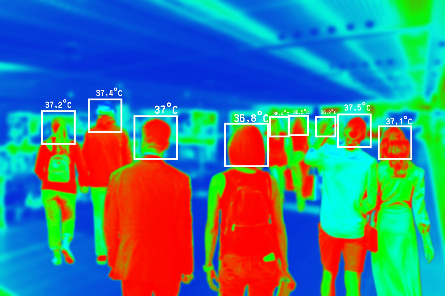

Feature extraction in computer vision turns raw pixel data into compact, descriptive representations that object detection, classification, segmentation and scene interpretation can work with. In practice the output is either a set of keypoints, each with a descriptor vector describing the patch around it, or one feature vector for the whole image taken from a trained network. Everything after that step depends on it: since features are the primitives later algorithms build on, the overall system is often only as good as its feature detector.
From pixels to feature vectors: what feature extraction in computer vision produces
A feature is information about the content of an image, usually about whether a certain region has certain properties. The same property can be represented in quite different ways. An edge can be a Boolean flag at each pixel, or a certainty measure combined with the edge’s orientation, and a region’s colour can be an average (three numbers) or a full colour histogram. When several kinds of feature are extracted at the same point, the usual practice is to stack them into a single feature vector.
The representation is a design decision with a cost attached. A more detailed description can be necessary to solve the problem, but it means more data and heavier processing. For matching, descriptors have to be distinctive enough to tell different 3D points apart while staying compact enough to store and compare cheaply.
Edges, corners, blobs and ridges: the structures extractors look for
A flat patch is hard to locate, and an edge can only be pinned down across its direction, because the pattern looks the same along it. A corner looks different wherever you move the patch, which makes it a good feature, and in some cases blobs are good features too. Harris and Stephens (1988) made this precise with the local auto-correlation function: two small curvatures mean a flat region, one high and one low curvature mean an edge, and two high curvatures mean a corner.
| Structure | Why it is useful (or not) | Typical detector |
|---|---|---|
| Flat region | Hard to localise; every shift looks alike | None |
| Edge | Localised across the edge only | Harris response with one dominant curvature |
| Corner / junction | Changes under any shift, so it can be found again | Harris auto-correlation matrix |
| Blob | Distinctive region with a characteristic size | Laplacian of Gaussian or its difference-of-Gaussian approximation; Hessian determinant in SURF |
| Ridge | Covered by the same scale-selection framework as blobs, corners and edges | Scale-selected differential operators |
Lindeberg’s scale-selection framework treats blobs, corners, edges and ridges in one way: local maxima over scales of normalised derivatives indicate how large a structure is. Getting this wrong has consequences, since descriptors can be highly unstable when computed at a badly chosen scale.
Is feature detection the same as feature extraction?
No. Detection decides where the interesting points are, and description characterises them. Feature detection finds the regions with maximum variation when shifted; description then summarises the region around each one so the same feature can be found in other images. Feature extraction usually means both phases together, and its result, after what can be considerable processing of the patch around each feature, is a descriptor or feature vector.
The pipeline for finding correspondences between images has three steps: select interest points, represent each neighbourhood as a descriptor, then match descriptors by a distance such as Euclidean. Detector and descriptor are judged on different criteria. A detector should be repeatable, finding the same physical points under different viewing conditions, while a descriptor should be distinctive and robust to noise and deformation.
| Stage | Question it answers | Output | Judged on |
|---|---|---|---|
| Detection | Where are the distinctive points? | Keypoints (location; in SIFT also scale and orientation) | Repeatability |
| Description | What does the region around each point look like? | Descriptor vector per keypoint | Distinctiveness, robustness, compactness |
| Matching | Which features correspond across images? | Pairs of matched features | Correct and false matches |
Lowe (2004) detects scale-space extrema of a difference-of-Gaussian, refines and filters them, assigns each keypoint an orientation, then builds a descriptor from local gradients. The descriptor is a 4x4 grid of 8-bin orientation histograms, giving 128 values per keypoint. In OpenCV that comes back as a list of keypoints plus a NumPy array of shape (number of keypoints) x 128.
Not every extractor works at sparse keypoints. HOG computes histograms of gradient orientation on a dense grid at a single scale, with no orientation alignment, and uses them as one long vector for the whole detection window, whereas SIFT descriptors are computed at sparse keypoints and used individually. A convolutional neural network goes further still and learns extraction and classification together, end to end, instead of keeping them as separate stages.
What classical extractors cost to compute
Classical extractors differ a lot from one another in cost. Lowe reports that a 500x500 image yields about 2000 stable SIFT features, depending on content and parameters, and that several thousand keypoints can be extracted in near real time on standard PC hardware. SURF was designed for speed: it uses integral images and a 64-dimensional descriptor instead of SIFT’s 128. Its authors measured detection and description of 1529 interest points at about 610 ms on a Pentium IV PC, and their fastest detector variant at more than five times the speed of difference-of-Gaussian.
ORB pushed further with a binary descriptor built on BRIEF, which Rublee et al. report as two orders of magnitude faster than SIFT while performing as well in many situations. Binary descriptors also need less storage and can be matched with Hamming distance, and descriptor dimension directly drives matching time.
If classical extraction is the bottleneck in a CPU-only deployment, the engineering options are covered in our article on accelerating CPU-bound classical CV feature extraction without a GPU.
Do SIFT and HOG still hold up against features learned by a CNN?
They hold up in controlled conditions and in reconstruction and localisation pipelines, and fall behind on semantic tasks with real-world variability. A 2026 facial-expression study shows the pattern clearly: HOG with an SVM reached 98.4% accuracy on the laboratory-controlled CK+ dataset, but its accuracy dropped significantly on FER-2013, which has uncontrolled lighting, pose, occlusion and background. An LBP texture descriptor with logistic regression did poorly everywhere, falling to 14.7% on KDEF. A lightweight CNN gave the best overall results, particularly on the harder data.
Razavian et al. took 4096-dimensional features from one layer of the OverFeat network, put a linear SVM on top, and reported consistently better results than highly tuned systems across object classification, scene recognition, fine-grained recognition and attribute detection. They concluded that deep convolutional features should be the primary candidate for most visual recognition tasks.
Matching and reconstruction are a different case. The Csurka, Dance and Humenberger survey (2018) found that learned descriptors reach the highest mean average precision on matching benchmarks, yet in image-based reconstruction and localisation pipelines handcrafted features perform as well or better. The HPatches benchmark found that a simple normalisation of traditional handcrafted descriptors can lift them to the level of learned descriptors under a realistic evaluation. In a periocular recognition study, combined traditional features (LBP, HOG, SIFT) scored between the CNNs and the ViTs, and adding them to fusions helped smaller models get close to the best results.
Our reading of this evidence is that the task decides. For recognising categories, expressions or identities under uncontrolled conditions, we would start from learned features. For geometric correspondence (stitching, pose estimation, reconstruction) on constrained imagery, a well-normalised SIFT pipeline is still a serious candidate, not a legacy fallback, and ORB earns its place where compute is tight. Handcrafted pipelines are lightweight and interpretable, which counts in resource-constrained settings, but their representational capacity is limited by their manual design. Those settings are where classical computer vision keeps its place in a system’s toolkit.
The choice also sits at a different level from tuning. Swapping HOG for pretrained CNN features changes what is computed, and we generally find that kind of restructuring offers bigger gains than optimising a fixed method.
Which pretrained models work as image feature extractors?
Most trained vision models can serve as image feature extractors. You remove the task-specific head and keep the outputs, and depending on depth those features range from edge- and corner-like responses to information about what real objects look like. In the feature-extraction approach the pretrained model stays frozen and only a new classifier on top is trained.
Which backbone? A 2023 evaluation of 16 pretrained models on four datasets found that CLIP-ResNet50, CLIP-ViT-B and ViT-H/14, the only three with transformer components, performed significantly better than the purely convolutional models on every dataset. Among the CNNs, ConvNeXt Large was best overall and AlexNet worst. Kornblith, Shlens and Le found a strong correlation between ImageNet accuracy and transfer accuracy when networks are used as fixed feature extractors (r = 0.99), but with two caveats. Some common regularisation methods slightly improve ImageNet accuracy while making penultimate-layer features much worse for transfer, and on two small fine-grained datasets ImageNet pretraining gave minimal benefit.
A clustering study found that the choice of CNN architecture had a huge impact on results for a given dataset, yet no pattern supported a rule like “for task T, use architecture A”. ViTs carry their own costs, including heavy training-data needs and compute.
Which layer to extract from
Early layers are general and higher layers specialise. Networks trained on natural images learn Gabor-like filters and colour blobs in their first layer, features that apply across many datasets and tasks, while higher layers specialise to the original task. For unsupervised clustering, the last layer before softmax gave the most discriminative features for every architecture and dataset tested.
That finding does not carry over to periocular recognition with ViTs. In the periocular study, ViT features peaked around layers 56 to 67 of 140 and were near optimal by layer 40, whereas CNNs needed nearly their full depth. The same authors found that the smaller ResNet18 came within 0.7 points of ResNet50’s 8.53% equal error rate, and that averaging feature vectors across channels, which is what a global-average-pooling output does, hurt accuracy. We would treat the layer as a parameter to sweep on your own data, starting from the penultimate layer for CNNs and from the middle for ViTs.
Doing it in torchvision and Hugging Face
In PyTorch, torchvision’s feature extraction utilities symbolically trace the model, set the nodes you select as outputs, remove everything downstream and return a new module. That lets you tap any intermediate layer of a backbone without rewriting it, for descriptors in retrieval or for feeding a feature hierarchy into a detection head. Image feature extraction as a task means removing a model’s task-specific head and using its features for similarity, retrieval or a new classifier.
How to tell whether a feature extractor is working for your task
Test the extractor on data that looks like deployment, with the metric your downstream task cares about. In the facial-expression study both HOG and the CNN were near perfect on CK+ and dropped noticeably on FER-2013, and its authors concluded that dataset complexity can affect performance more than the choice of representation alone. Near-perfect accuracy on a controlled dataset does not imply real-world generalisation.
A checklist we would run before committing to an extractor:
- Hold out realistic data. Include the lighting, pose, occlusion and background variation of the target environment, since controlled-set accuracy does not imply real-world generalisation.
- Measure detector repeatability for keypoint pipelines: the share of points found again at a matching location and scale after known transformations, as in Lowe’s protocol.
- Score the downstream task with a simple head. A frozen extractor with a newly trained output layer gives a simple probe; the studies above report NMI or clustering accuracy for clustering, equal error rate for periocular recognition and mean average precision for matching.
- Fix the evaluation protocol. HPatches was built because existing datasets left evaluation details ambiguous and produced inconsistent results across papers.
- Compare several extractors, and their combination. Different pretrained CNNs carry complementary information, and combining them raised clustering accuracy and lowered variability; fusing CNN and ViT features also lowered error in the periocular study.
- Check normalisation before blaming the method. Per-channel L2 normalisation gave the best accuracy for CNN features in one study, and normalisation alone brought handcrafted descriptors level with learned ones on HPatches.
- Measure compute cost alongside accuracy, because the descriptor and backbone choices above differ in compute.
One question remains open, and the literature does not settle it. Researchers can show that the extractor has a major effect on results, but not how to pick the right one in advance, and a 2023 evaluation of pretrained extractors reached the same conclusion: different models win on different datasets, so candidates have to be tested systematically against the target data. That makes the evaluation harness, not the backbone, the part of a vision system to build first. It is also where computer vision R&D work at TechnoLynx connects extractor choice to the rest of the pipeline.