The emergence of DALL-E [3], Stable Diffusion [4] and other similar models in recent years have taken the world by storm with their unparalleled image synthesis capabilities, surpassing the quality produced by traditional methods such as Generative Adversarial Networks (GANs), Normalizing Flows, and Variational Autoencoders (VAEs). DALL-E’s innovative approach to image synthesis has placed it at the forefront of the field, captivating the mainstream consciousness and setting a new standard for what is possible in this area of artificial intelligence.
In this article, we will delve into the underlying concepts of diffusion networks and provide a practical explanation on how such a model can be trained and used to generate novel images. By the end of this article, you will have a clear understanding of the intuition behind diffusion networks and a step-by-step procedure for using them for image generation.
Introducing Diffusion Models
Diffusion models are a type of probabilistic generative model [6] that use and generate new, high-quality data that resembles the original input. This approach is useful for tasks such as denoising and data generation, as it can be trained to preserve the underlying structure of the data while removing or reducing unwanted noise.

Diffusion models can be understood as a type of latent variable model, where the term “latent” refers to the presence of a hidden continuous feature space. The mapping from the original image to this latent space is achieved through a Markov Chain, which is essentially a series of T timesteps that add random noise to the image at each step. This process follows the Markov property, meaning that the next time step is only dependent on the previous one. These diffusion models are a way to incorporate uncertainty into the mapping from the original image to the latent space, leading to more robust and flexible models.
Diffusion models are made up of two main processes:
- The forward process: It starts out at with the original image x₀ and at every step, some noise is added to it until the image turns into pure noise.
- Parametrized Backward process: In the backward process the model is tasked with predicting the noise that has been added to the images between each step. It is called parametrized because we use a neural network for this part. If we succeed in training a network to predict the noise, we can then use it to generate new images from pure noise by predicting and removing this noise, then iteratively progressing up until x0 is reached.

It is important to note that unlike with VAEs, the input image and latent variable dimension match, which lends U-Net architecture as a fitting choice for the noise predictor.
Forward diffusion process
The main objective of the forward process is to add noise to the image, which mathematically can be written as:
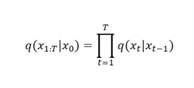
Where x0 is the initial input, and as this is a Markov chain, each subsequent output is only dependent on the sample that came before it.
The Gaussian noise added between each step can be written as:


βₜ is called the variance schedule and it controls the amount of noise we add to the image at each timestep. As t grows so does βₜ meaning the 1 — βₜ term decreases until the mean of the sample reaches 0. I is the identity matrix, this means that the variance is fixed. Although there are variations of diffusion networks where the model learns the variance of the noise as well, for the sake of simplicity we stick to a version where it is fixed and only the mean is learnt.
Choosing a suitable βₜ is called noise scheduling, and it is very important as we want to set it in a way that the image at time T just about reaches a 0 mean, 1 variance Gaussian. If this happens too early or too much information remains at step T, training can fail, and our model will not converge properly.
There are many different strategies for noise scheduling [1] such as:
- changing the noise schedule functions: linear, cosine, cosine (logSNR), sigmoid, sigmoid (logSNR), quadratic.

- adjusting the input scaling factor b in the following equation for the sample:

Lastly, even though we talk about iteratively noising images in the forward process, it is important to point out that because the sum of Gaussians is still a Gaussian, we can actually sample the noised image at timestep t immediately without having to go through all the previous steps thanks to the reparameterization trick.

In another form this can be written as:

In this case, we need to pre-calculate αₜ the so-called cumulative variance schedule based on the following equations.

Backward denoising process
The backward step of the process is used in two different ways: to train the model and to generate new images from noise (this is referred to as sampling).

During training, we don’t iterate over every timestep, instead, we choose a random t, sample some noise, ϵ and use it in the forward process that we already discussed to get the noisy sample xₜ We can feed this noisy image into our neural network that will predict the noise that was used to generate the image. The loss will be the L2 distance between the predicted and the real noise.
When we want to create a completely new image from noise, we must start from xₜ (pure noise) and iterate over every timestep, passing our noisy image into the trained network that will predict the noise ϵ which we can use to calculate the noise for the current timestep, which is then deducted from the current image xₜ to get xₜ ₋ ₁ until we reach x₀.
Architecture
As we already stated, a U-Net [5] is adequate for predicting the noise from an input image as it has the same input and output dimensions and has been an imperative component not just in image segmentation tasks but also in synthesis in GANs and its conditional variants as well.
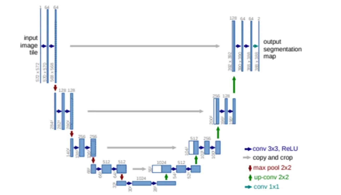
The main feature of a U-Net is its hierarchical nature in which the input images go through a set of down-sampling layers where at every step, the image loses spatial information but gains feature channels. At the bottom, the data reaches a bottleneck which is followed by a series of up-sampling layers that increase the image size but reduce the depth of the data. Furthermore, residual connections can be found between every up and down-sampling module of the same size. In addition to these basic features in more recent networks, attention layers are also used as these can help the network focus on the more interesting parts of the image.
The Math
The reverse process can be described mathematically with the following equations:

We start from pure noise with 1 variance and mean 0. The following formula describes how the model learns the probability density of the previous timestep given the current one.

This density ρθ is defined by the predicted Gaussian noise distribution in the image, to get the previous step xₜ ₋ ₁ we need to remove this noise from xₜ
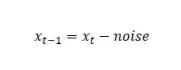
The complete formula for calculating xₜ ₋ ₁:

Here ϵθ is the output of the U-Net, which tries to predict the ϵ that we used in the forward process to generate xₜ. The σₜz part is another Gaussian noise we generate to then inject into the update to avoid collapses into local minima. This comes from stochastic gradient Langevin dynamics which is a concept from physics for the statistical modelling of molecular systems.
Timestep Encoding
Timestep Encoding is also an important topic to touch on. This is because we use the same U-Net across all timesteps, meaning weights are shared, so we need to somehow tell our model at which timestep it’s currently working. To do this, we typically use something called positional embedding, which is used to encode discrete positional information along with our data. The purpose of positional embedding is to assign a unique vector for every index.
Encoding for the kₜₕ object in a sequence of L size can be done using the following equations:
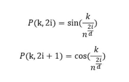
The explanation for the different variable is as follows:
- k: position of an object in the input sequence, also 0 ≤ k <L/2
- d: dimension of the output embedding space
- P(k,j) position function for the mapping
- n: arbitrary scalar: usually 10000
- i: column index of the encoding matrix 0 ≤ i <d/2
In this case even positions (in the encoding matrix) will be used with the sine wave and odd positions will be encoded with the cosine wave.
The advantages of encoding positions like this are as follows:
- Both sine and cosine take up values between [-1,1], meaning the encoding matrix is always normalized.
- As the sinusoid for each position is different, each k is encoded to a unique vector.
- In the case of natural language processing tasks, this enables the measurement of similarity between each position for the relative position encoding of words.
If we plot the embedding matrix with the y axis as k and the x axis as i we get the following graph:
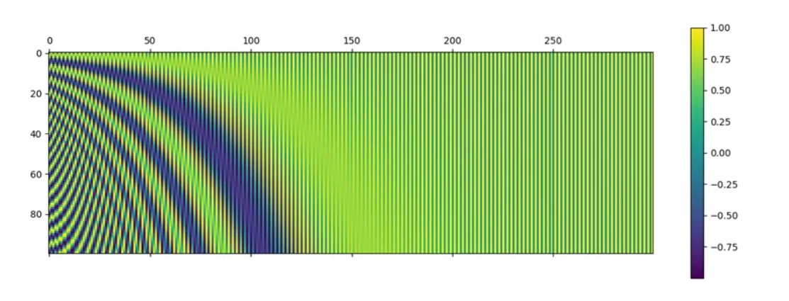
For k=0 position’s embedding vector would simply be the first row of this graph, k=1 the second and so on.
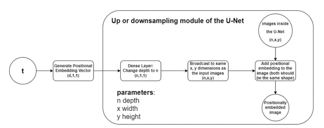
The way these embeddings are used in the U-Net is that for a given timestep, we generate the positional embedding vector based on the formulas presented above, send it through a dense layer to achieve the same feature depth as the images at that current level, and finally, these vectors are broadcasted to each x and y position and simply added to the images both during up and down-sampling.
Loss metric
The researchers in [2] used the variational lower bound to optimize their model, akin to VAEs. The first loss term they derived for the model used the mean and predicted mean of the sample:

Afterwards, they reparametrized the Gaussian term to predict epsilon from the input xₜ at timestep t because xₜ is available as input during training time.
We know that:
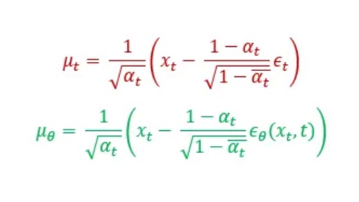
If we substitute these into the previous formula:
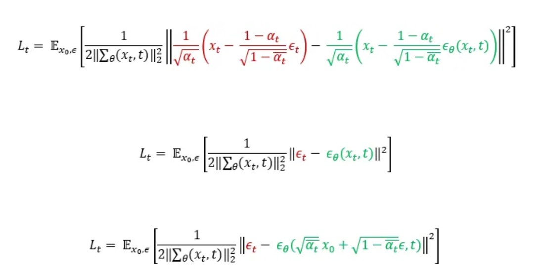
Lastly [2] found that the training worked better with a simplified objective where they remove the weighting term, which leaves the following final formula:

This means that in order to train the U-Net, the loss we have to calculate is simply the squared error between the predicted noise ϵθ, which is the direct output of the model and the real noise ϵ that we sampled when generating xₜ.
While this result might seem quite straightforward, the mathematical derivations behind it are far from simple. In fact, they can be quite complex so for those who are interested in delving deeper into the math side of things, the website provides a detailed explanation of the process.
Our Opinion
Here at TechnoLynx we encounter a wide variety of image processing problems that can be solved with anything ranging from traditional algorithms to complex neural networks. Diffusion networks will complete our machine learning toolset that we can leverage to generate images at a quality that is unparalleled by any other network we’ve encountered. While it might not be as fast in terms of inference as a GAN, the diffusion training process is stable and not prone to the same pitfalls as adversarial models. This means quicker, safer results and a more robust development process for our team. We at TechnoLynx are certainly looking forward to seeing what the future holds for this technology.
This has been an interesting high-level look of the model, but we are not done yet. Our next plan is to investigate how such a model can be converted to Core ML using coremltools for Apple devices. If you liked this article and would like to learn more, please follow us on Medium here and be sure to check out our website.
References
- [1] Chen, T. (2023). On the Importance of Noise Scheduling for Diffusion Models
- [2] Ho, J., Jain, A., & Abbeel, P. (2020). Denoising Diffusion Probabilistic Models
- [3] Ramesh, A., Pavlov, M., Goh, G., Gray, S., Voss, C., Radford, A., . . . Sutskever, I. (2021). Zero-Shot Text-to-Image Generation
- [4] Rombach, R., Blattmann, A., Lorenz, D., Esser, P., & Ommer, B. (2022). High-Resolution Image Synthesis with Latent Diffusion Models
- [5] Ronneberger, O., Fischer, P., & Brox, T. (2015). U-Net: Convolutional Networks for Biomedical Image Segmentation
- [6] Yang, L., Zhang, Z., Song, Y., Hong, S., Xu, R., Zhao, Y., . . . Yang, M.-H. (2022). Diffusion Models: A Comprehensive Survey of Methods and Applications

