With the hype of generative AI, all of us had the urge to build a generative AI application or even needed to integrate it into a web application. To fulfil these urges, we decided to pick the task of generating human faces using a Variational Autoencoder and then implement the needed back-end/front-end for it to run online. The built web app can generate high-resolution faces and combine features from two generated faces into one using interpolation; thus, it was named Face Mixing. This article describes the technical challenges we faced and how we overcame them.

What is an Autoencoder?

An Autoencoder is a neural network model consisting of two parts: an encoder and a decoder. The encoder aims to take samples from a high-dimensional input space and project them onto a lower-dimensional space, ultimately encoding the data into a compressed representation. This lower dimensional space is what we call the latent space. On the other hand, the decoder aims to reverse this projection. It takes samples from the latent space (latent vectors) and projects them back onto the input space. The architecture of a simple autoencoder is shown below.

A diagram of simple autoencoder architecture

Before training, these projections are initialized randomly. Training brings these projections as close to being each other’s inverses as possible. To achieve this, we considered the encoder and the decoder as if they weren’t separate but one connected model. The encoder’s output is fed directly to the decoder, keeping track of the gradients in both. To ensure the decoder is reconstructing an accurate version of the original input, the loss function is as simple as an L1 or L2 between the encoder’s input and the decoder’s output. Thus, the training is semi-supervised; hence, the dataset can be pretty simple, requiring only some raw data without labels or annotations.

A sample of the training code in TensorFlow for one batch of data is shown below:

@tf.function 
def train_for_one_batch(batch): 
        with tf.GradientTape() as tape_encoder, tf.GradientTape() as tape_decoder: 
            latent = encoder(batch)  
            recon = decoder(latent) 
            loss_value = loss_fn(batch, recon) 
 
        gradients = tape_decoder.gradient(loss_value, decoder.trainable_weights) 
        optimizer.apply_gradients(zip(gradients, decoder.trainable_weights)) 
        gradients = tape_encoder.gradient(loss_value, encoder.trainable_weights) 
        optimizer.apply_gradients(zip(gradients, encoder.trainable_weights)) 

Transitioning from Autoencoder to VAE

A simple Autoencoder has no restrictions on the shape of the latent space. It is merely decided by the model, which is convenient to implement but has drawbacks. For example, the areas where the latent space produces a viable output are undetermined. If we are to sample a random latent vector from the latent space, chances are high that the output would be incomprehensible. Aiming to create a generative model, this is a highly unwanted property.

The Architecture of a Simple VAE

The solution is to use Variational Autoencoders (VAE). A VAE makes the simple Autoencoder stochastic. Rather than a single latent vector, the encoder outputs a Gaussian distribution. This distribution is characterized by its mean and the logarithm of its variance.

But how to pass such a distribution to the decoder?

Since the gradient flow can not handle stochasticity, the trick we use is called the reparameterization trick. It simply means taking a sample from the Gaussian distribution that was the encoder’s output. Then, the obtained latent vector is passed into the decoder.

The training loop is modified slightly; we add another loss term, the KL divergence loss. This aims to push the encoded distribution towards the standard normal distribution. This modification is suitable for our purpose because:

• The decodable latent vectors are all around 0.
• If we take two latent vectors and start to interpolate between them, due to the distributions being close to standard normal, we see that the decoded outputs are mixtures of the two data points in some abstract sense. For example, if one input is a picture of a woman, the other is a picture of a man, and we start interpolating between their corresponding latent vectors, we get faces that are half man, half woman. This property is what we use extensively in our Face Mixing web app.

A sample of the VAE training code in TensorFlow for one batch is shown below.

@tf.function
deftrain_for_one_batch(batch):
withtf.GradientTape() astape_encoder, tf.GradientTape() astape_decoder:
mean, logvar = encoder(batch)
latent = reparameterize(mean, logvar)
recon = decoder(latent)
loss_value = loss_fn(batch, recon, mean, logvar)

gradients = tape_decoder.gradient(loss_value, decoder.trainable_weights)
optimizer.apply_gradients(zip(gradients, decoder.trainable_weights))
gradients = tape_encoder.gradient(loss_value, encoder.trainable_weights)
optimizer.apply_gradients(zip(gradients, encoder.trainable_weights))

Limitations of VAEs

VAEs are not a new technology but are surpassed by other generative models such as VAEGANs and diffusion models. Yet, VAEs’ most significant selling point is that they are usually much smaller models than their competitors. Whereas a decent stable diffusion model takes up around 10 GB of memory, a trained VAE for our use case fits into a couple of tens of megabytes.

However, choosing VAE comes with limitations to overcome. The hardest one of these limitations is that a VAE (just like a simple Autoencoder) tends to produce blurry images; it has a hard time learning high-resolution details.

To overcome this limitation, we investigated newer tricks used for state-of-the-art models and ported whatever we could to the VAE. These modifications are discussed later in the article.

The used data

The Face Mixing web app aims to create reasonably high-resolution images of faces with high-level detail present. The image size has to achieve a good balance between resolution, the processing power, and the model size needed to generate them. We decided to use 256x256 images.

Since VAEs are semi-supervised models, we only needed to collect images of faces in the desired resolution without annotation. Our dataset contains 30,000 images.

Our data-loading process was simple and can be defined using the following lines.

class DataLoader: 
    def __init__(self, data_dir, image_size, batch_size): 
        self.data_dir = data_dir 
        self.data_files = np.array([os.path.join(data_dir, file) for file in os.listdir(data_dir)]) 
        self.batched_data_files = [] 
        self.image_size = image_size 
        self.batch_size = batch_size 
        self.index = 0 
        self.num_batches = -1 
        self.data_end = True 
 
def init_dataloader(self): 
    np.random.shuffle(self.data_files) 
    self.batch_data_files() 
    self.num_batches = len(self.batched_data_files) 
    self.index = 0 
    self.data_end = False

The DataLoader class listed all the image file names in the list data_files. When the init_dataloader() function is called, these file names would be organized into batches and be written into the batched_data_files list. Then, the index variable is used to traverse this list. Moreover, at each call of the load_next_batch function, all the files are loaded in the next batch of file names and returned as floating-point images with values between -1 and 1.

def load_next_batch(self):
    out = []
for file in self.batched_data_files[self.index]:
img = cv2.imread(file)
img = img.astype(np.float32) / 128 - 1
out.append(img)

self.index += 1
if self.index == self.num_batches:
self.index = -1
self.data_end = True

return np.array(out)

The faces encoder

Our choice for the encoder does not have a very complex architecture, as the encoder’s job is usually much easier than the decoder’s. We used a mostly convolutional network for a basic encoder architecture with two tricks: batch normalization and spectral normalization. Batch normalization is widely used in many machine learning problems to make the training more stable, allowing higher learning rates. Meanwhile, spectral normalization was initially used for GANs to stabilize their training and reduce the chance of mode collapse. It does not apply normalization to the data; instead, it controls the layer weights where it is applied.

We set the latent space to have a dimensionality of 1×256. The model has two outputs, the mean and the log of the variance of the Gaussian over the latent space; both are 256-long vectors.

The face encoder architecture

The faces decoder

The decoder model has a high complexity level, which received many modifications and updates compared to a base VAE’s decoder architecture. In principle, it receives a latent vector, uses a dense layer to increase its dimensionality, reshapes it to two dimensions, and then applies the decoder block. Each decoder block increases the resolution by a factor of 2 on both axes, eventually reaching the original 256x256 resolution.

The face decoder architecture

The content of the Decoder Block

In addition to the spectral normalization, the first trick we implemented to improve training stability and the reconstruction’s high-level detail was making the decoder output multi-scaled. In each decoder block, we extract an output image at the current resolution with a simple out-convolution and return each output from the model. We apply an l1 loss function at each level, meaning that the model receives gradients at the top level and in multiple places, which results in a more controlled training process.

A general issue with autoencoders is that the decoder can sometimes “forget” the latent vector during reconstruction. It uses the information coded in the latent vector only at the low-resolution levels and acts as a basic upsampler at higher-resolution levels. Hence, this partially causes the blurry outputs. To improve the output resolution we implemented a custom renormalization step, which is a function of the latent vector. For the batch normalization, we disabled the automatic recentering and rescaling at each level. Instead, we extracted the beta and gamma parameters from the latent vector using dense layers and applied them manually. This modification reintroduces the latent vector at each level of the reconstruction so that the model cannot forget it. The code snippet below implements this custom renormalization.

res = BatchNormalization(center=False, scale=False)(res)

common_dense = SpectralNormalization(Dense(channels * 4, activation='leaky_relu', kernel_initializer='he_normal'))(lv)
common_dense = BatchNormalization()(common_dense)
beta = SpectralNormalization(Dense(channels, kernel_initializer='he_normal'))(common_dense)
beta = Reshape((1, 1, channels))(beta)
gamma = SpectralNormalization(Dense(channels, kernel_initializer='he_normal'))(common_dense)
gamma = Reshape((1, 1, channels))(gamma)
res = res * (1 + gamma) + beta

The training process

Our training process is close to the example VAE training loop introduced above. However, we did make some important modifications to the loss function.

@tf.function
def loss_fn(x, recons, mean, logvar):
loss_dict = {}
    l1_loss = tf.keras.losses.MeanAbsoluteError()

# reconloss
recon_loss = 0
x_copy = tf.identity(x)
for level in recons[::-1]:
recon_loss += l1_loss(level, x_copy)
x_copy = tf.image.resize(x_copy, (x_copy.shape[1] // 2, x_copy.shape[2] // 2), method='bicubic')
recon_loss /= len(recons)
loss_dict["l1"] = recon_loss

# kldivergenceloss
kld_loss = -0.5 * tf.reduce_sum(1 + logvar - tf.pow(mean, 2) - tf.exp(logvar))
kld_loss /= BATCH_SIZE
loss_dict["kld"] = kld_loss

# vggloss
vgg_loss = 0
vgg_input_x = (x[..., ::-1] + 1) * 128
tf.keras.applications.vgg19.preprocess_input(vgg_input_x)
vgg_x = vgg19(vgg_input_x)
vgg_input_recon = (recons[-1][..., ::-1] + 1) * 128
tf.keras.applications.vgg19.preprocess_input(vgg_input_recon)
vgg_recon = vgg19(vgg_input_recon)
for i in range(len(vgg_x)):
vgg_loss += l1_loss(vgg_x[i], vgg_recon[i])
vgg_loss /= len(vgg_x)
loss_dict["vgg"] = vgg_loss

loss = RECON_LOSS_MULTIPLIER * recon_loss + VGG_LOSS_MULTIPLIER * vgg_loss + KLD_LOSS_MULTIPLIER * kld_loss
return loss, loss_dict

In the code above, x is the original input image, recons is a list of all the different resolution outputs from the decoder, and mean and logvar are the encoder outputs. First, we calculate the l1 reconstruction loss at each output resolution. We downsample the original image to the required resolution at each step. Then, we calculate the KL divergence loss. Finally, we apply a perceptual loss to the highest resolution output, which brings us to our final modification of the base VAE.

Using purely l1 loss tends to push the model towards generating blurry images since a blurry representation of the input still results in low loss scores. On the other hand, perceptual losses aim to compare images in abstract ways that better resemble human vision. The perceptual loss we implemented runs a pre-trained VGG model on the original image and its reconstruction, extracts multiple outputs from different VGG layers, and compares the original and reconstruction for each output vector.

The selection of the desired output layer from the VGG model is done using the code below:

vgg19 = VGG19(include_top=False, weights='imagenet', input_shape=(IMAGE_SIZE, IMAGE_SIZE, 3))
vgg19_selectedLayers = [1, 2, 9, 10, 17, 18]
vgg19_selectedOutputs = [vgg19.layers[i].outputfori in vgg19_selectedLayers]
vgg19 = Model(vgg19.inputs, vgg19_selectedOutputs)

The addition of the perceptual loss made a substantial difference in the presence and quality of high-level details in the generated images.

Converting the model to TensorFlow JS

TensorFlow JS (tfjs) runs the model in the browser on the client side. Thus, we must convert our Keras model to run it in tfjs. The tfjs_converter script is used, which is included with TensorFlow JS. The only problem is that tfjs’s functionalities are limited compared to TensorFlow’s Python version. One of these limitations was that tfjs does not recognize the spectral normalization layer.

Thankfully, spectral normalization only affects the model during training; it has no effect at inference time, so our solution is to utterly remove the Spectral Normalization wrappers from the layers using the script below. It creates a new model with the same architecture as the original decoder, missing the spectral normalization wrappers. Then, it goes through all the layers and sets the weights of the new model to the exact weights of the trained model. After running this script, we can convert the model using tfjs_converter.

model = keras.models.load_model("decoder") 
model2 = decoder_model_no_spectral(256) 
 
for i in range(len(model.layers)): 
    if not model.layers[i].get_weights(): 
        continue 
    if model.layers[i].__class__.__name__ == 'SpectralNormalization': 
        layer = model.layers[i].layer 
    else: 
        layer = model.layers[i] 
    model2.get_layer(layer.name).set_weights(layer.get_weights()) 

Loading the model

With the growing number of users, running the models on the server side would result in a long waiting time for simple requests. To solve this, we can run the model on the client side, which also helps to make it available even during network disruptions. The simplest way to load the model after conversion is to use the loadGraphModel function with the following script:

const model = awaittf.loadGraphModel('path/to/model.json ');

Latent storing

Matching a latent vector to a set of known features is an easy task. Mathematically, isolating a feature and calculating its latent vector are achieved by averaging an abundance of latent vectors belonging to different faces sharing this exact feature. Yet, ensuring feature isolation requires identicality between the original faces (input of the encoder) and the generated faces (output of the decoder), and this is impossible using the selected generative approach. Hence, a dataset is generated connecting the features present in a face with its encoding result as a latent vector. We chose 5,000 images of different faces with diverse features that formulate multiple options for the user to select from in the UI. The dataset generation is automated, and the latent vectors accompanied by their associated features are saved in a CSV file that is handled by the back-end code.

Feature selection

To generate faces, users can choose the features they want to see on the final image. However, those features must be matched into a latent vector serving as a decoder input. Thus, we create a binary vector where each element corresponds to a feature in the user input. If the feature was selected on the UI, the element value is 1; otherwise, it is 0. From the latent vector generation, we have a correspondence of feature vectors to the latent ones, and we can use it to find all possible latent vectors corresponding to a user’s input. If the user-chosen feature combination (features vector) is not included in the stored latent vectors, some chosen features are skipped, and the generated image is missing them accordingly. Whenever this happens, a message indicating the case with the missing features is displayed.

The offered features set for selection

Face generation

Taking the latent vector from the previous step as a decoder input, we receive a 1d vector representing an image. It stores the value for all 3 RGB colors for each image pixel. To display it, we start with the image creation and then modify its data according to the values in the model output.

var canvas = document.getElementById(your_image_placeholder_id);
var ctx = canvas.getContext("2d");
var image = ctx.createImageData(1, 1);     
for (let y=0; y<img_length; y++) {
for (let x=0; x<img_width; x++) {
let b = img_from_decoder[(y*img_width + x)*3 + 0];
let g = img_from_decoder[(y*img_width + x)*3 + 1];
let r =img_from_decoder[(y*img_width] + x)*3 + 2];
            if (isNaN(r) || isNaN(g) || isNaN(b)) {
image.data[0] = (x+2*y) % 256;    // Red
image.data[1] = (x+3*y) % 256;    // Green
image.data[2] = (x+5*y) % 256;    // Blue
} else {
image.data[0] = Math.max(0, Math.min(255, (r + 1)*127));    // Red
image.data[1] = Math.max(0, Math.min(255, (g + 1)*127));    // Green
image.data[2] = Math.max(0, Math.min(255, (b + 1)*127));    // Blue
            }
image.data[3] = 255;                                // Alpha
ctx.putImageData(image, x, y);
}
 }

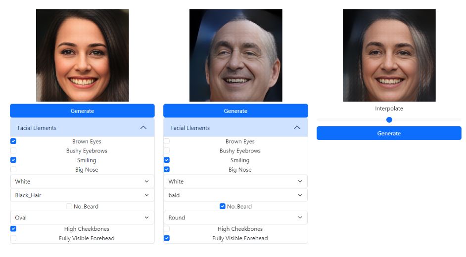
For example, we can generate aface by selectinga set offeatures,as shown below. Yet, selecting the same features would not always generate the same Face.

generative AI

The interpolation functionality

The number of latent vectors may limit the number of generated images. The solution for avoiding this limitation is interpolating already generated images. After having two generated faces, a user can use a slider to choose the ratio between them in the interpolated image. This is done by calculating a new latent vector using the formula in the code below:

interpolation_latent = weight*img1_latent + (1-weight)*img2_latent, where 0 <= weight <= 1, slider value

Having a latent vector, we can generate a new face, a mixture of two previous as we see below.

generative AI

Conclusion

At the end of this article, we hope that you enjoyed reading our detailed description of how to build the Face Mixing web app and how we overcame multiple challenges. Don’t forget to check out the complete code, which is available publicly on GitHub.

A shout-out to our brilliant R&D engineers who helped write this article, Ákos Rúzsa and Oleksandra Tsepilova.

Make sure to give this Face Mixing demo a try on our website.

You may also compete against our AI Chess engine using hand gestures. For more information, refer to our article on how we built the simple version of this chess game. For more exciting articles on similar topics, make sure to follow us.