Introduction to Logistics Routing and Distribution Challenges

Within the logistics and supply chain industry, intelligent routing is key for delivering products to customers faster and more cost-effectively. Different modes of distribution, such as road, rail, air, and sea, play an important role in logistics planning. Each mode has its advantages, depending on factors like distance, cost, and delivery time. Currently, road transportation is responsible for 53% of global CO2 emissions, and organisations worldwide are facing growing pressure regarding improving delivery management.

According to McKinsey’s 2022 report, the road freight market is expected to grow by 6.03% each year until 2027. As the market grows, the need for greener solutions makes efficient routing more critical than ever.

Some significant challenges include cutting down fuel use, meeting tight delivery deadlines, and planning routes that are better for the environment. The boom in online shopping has added further pressure as customers increasingly expect same-day delivery. Over 51% of retailers currently offer same-day delivery, and by 2024, this number could hit 99%.

A major obstacle to addressing these challenges is solving the Vehicle Routing Problem (VRP). The VRP is a complex optimisation task that involves finding the most efficient routes for a fleet of vehicles to deliver goods to multiple locations. Given its complexity, finding practical solutions for routing and distribution is crucial. In this article, we will explore various approaches and techniques to solve the VRP, including real-world examples and a step-by-step coding tutorial.

A brief timeline of routing optimisation and VRP. Source: DistanceMatrix

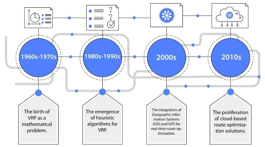
Understanding the Vehicle Routing Problem (VRP)

The Vehicle Routing Problem focuses on finding the most cost-effective routes for a fleet of vehicles to deliver goods to multiple customers. The VRP plays an essential role in logistics by impacting the efficiency of distribution networks. As an NP-hard (Nondeterministic Polynomial time) problem - meaning it’s computationally difficult to solve exactly as the problem size increases - solutions often rely on heuristic approaches, which provide practical, though not always optimal, solutions. A heuristic solution to the VRP generally takes into account factors like fuel, distance, and time. Efficiently solving the VRP helps companies save money, reduce delivery times, and keep customers satisfied.

=An example of a VRP where each node is visited once by a single vehicle starting and ending at a central depot. Source: AWS Amazon

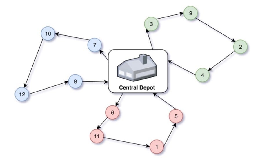
There are several types of VRPs, each with its own challenges. These variations address different needs and constraints in routing:

• Travelling Salesman Problem (TSP): In this version, the goal is to find the shortest route for a salesperson (or a delivery vehicle) to visit several stops and return to the starting point. The more stops there are, the harder it becomes to arrive at the best route.

• Capacitated VRP (CVRP) takes into account each vehicle’s capacity. The challenge is to plan routes that complete all deliveries while staying within each vehicle’s weight or size limit.

• VRP with Time Windows (VRPTW): Each customer has a specific delivery time slot in this variation. The challenge is to plan routes that manage the vehicle’s load while meeting these time constraints.

An example of a vehicle routing problem with time windows. Source: Altamira

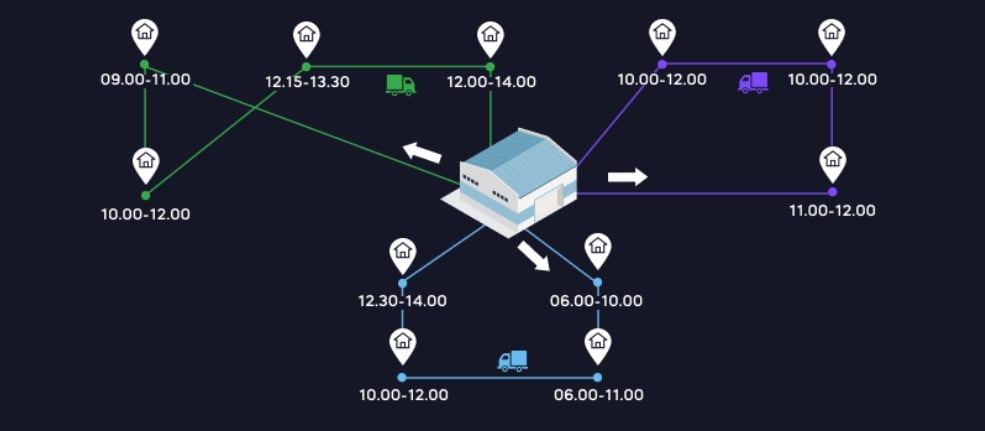
Solving the VRP helps create efficient delivery routes, reduce fuel consumption, and cut logistics costs. It also lowers businesses’ environmental impact by reducing the number of vehicles on the road.

Several algorithms can be applied to solve the VRP. Here are some of the most interesting solutions:

• Genetic Algorithms: Inspired by the process of natural evolution, these algorithms search for the best possible routes. They do this by iteratively combining and mutating a population of potential solutions to evolve towards an optimal or near-optimal solution over generations.

• Ant Colony Optimisation: By mimicking how ants find the shortest path to food, this approach helps discover the most efficient routes. It relies on positive feedback mechanisms that reinforce successful paths, allowing the algorithm to converge more quickly to the best solution.

• Simulated Annealing: This approach explores different solutions and occasionally accepts less optimal ones to avoid getting stuck in local minima. By gradually reducing the “temperature,” it decreases randomness over time and enables convergence towards an optimal solution.

Another practical way to solve VRP is by using tools like Google OR-Tools with Python. These tools provide ready-made algorithms to optimise routes and make it easier for companies to implement VRP solutions. They can handle various challenges, such as delivery time windows and vehicle capacities, to suit different business needs. Additionally, they are flexible and customisable, so companies can fine-tune solutions to their specific requirements, improve route planning, reduce travel distances, save on fuel costs, and boost overall efficiency.

Step-by-Step Coding Tutorial: Solving VRP Using Python and Google OR-Tools

In this tutorial, we will explore how to solve the Vehicle Routing Problem (VRP) using Python and Google OR-Tools. We will work with a real-life logistics scenario. Let’s say a manufacturer needs to transport raw materials from multiple suppliers to various production facilities and wants to optimise these routes to ensure timely and cost-effective deliveries.

Setup and Prerequisites

Before diving into the code, we need to make sure that everything is set up properly. Follow these steps to install and configure the required tools.

• Install Python: Ensure you have Python installed (version 3.7 or higher).

• Install Google OR-Tools: OR-Tools is Google’s open-source software suite that provides tools for solving optimisation problems, including VRP. To install it, open your terminal and run:

pip install ortools

Defining the Problem

In this scenario, the goal is to optimise the routes for a fleet of vehicles delivering materials from a distribution centre to multiple suppliers and production sites across major cities in the United States. The objective is to minimise travel distances and costs while adhering to vehicle capacity and time constraints.

In this tutorial, we’ll solve a simplified version of the VRP:

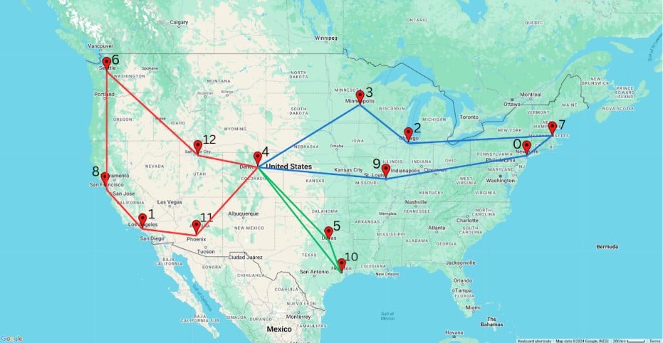
• Distribution Centre (Depot) and Multiple Delivery Points: The depot is centrally located in Denver, Colorado, with delivery points in major US cities like New York, Los Angeles, Chicago, and others.

• A Fleet of Vehicles with Specific Capacities: Three vehicles start from the depot and deliver goods to various cities, efficiently using their capacities while minimising the total distance.

• Distance Matrix Representation: A distance matrix defines the distances (in miles) between cities and is used to calculate the optimal routes for the fleet.

Input Data Required

To solve this problem, we need the following input data:

• Distance Matrix: A matrix where each element represents the distance between two locations.

• Number of Vehicles: The total number of vehicles available in the fleet.

• Vehicle Capacities: The maximum load each vehicle can carry.

• Depot: The starting location (or distribution centre) where all the vehicles begin and end their routes.

Implementing the Solution

Next, we’ll discuss the process of solving VRP using Python and Google OR-Tools.

Data Preparation

Defining Locations. Source: TechnoLynx

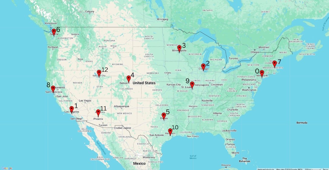
To solve the problem, we first need to define the locations, the distance matrix, and other constraints. For this, a function is created to encapsulate all the necessary information.

The following code imports the required modules, and the create_data_model() function is used to set up a data model that includes a distance matrix (a nested list showing the distances in miles between different locations). For example, it indicates that the distance between New York and Los Angeles is 2,451 miles.

The function also specifies the number of vehicles available (num_vehicles = 3) and sets the depot (starting point) for all vehicles to the location at index 4 in the matrix.

from ortools.constraint_solver import routing_enums_pb2
from ortools.constraint_solver import pywrapcp

def create_data_model():
   """Stores the data for the problem."""
   data = {}
# Distance matrix (in miles)
   """
0. New York - 1. Los Angeles - 2. Chicago - 3. Minneapolis - 4. Denver - 5. Dallas - 6. Seattle - 7. Boston - 8. San Francisco - 9. St. Louis - 10. Houston - 11. Phoenix - 12. Salt Lake City
   """
   data["distance_matrix"] = [
       [0, 2451, 713, 1018, 1631, 1374, 2408, 213, 2571, 875, 1420, 2145, 1972],
       [2451, 0, 1745, 1524, 831, 1240, 959, 2596, 403, 1589, 1374, 357, 579],
       [713, 1745, 0, 355, 920, 803, 1737, 851, 1858, 262, 940, 1453, 1260],
       [1018, 1524, 355, 0, 700, 862, 1395, 1123, 1584, 466, 1056, 1280, 987],
       [1631, 831, 920, 700, 0, 663, 1021, 1769, 949, 796, 879, 586, 371],
       [1374, 1240, 803, 862, 663, 0, 1681, 1551, 1765, 547, 225, 887, 999],
       [2408, 959, 1737, 1395, 1021, 1681, 0, 2493, 678, 1724, 1891, 1114, 701],
       [213, 2596, 851, 1123, 1769, 1551, 2493, 0, 2699, 1038, 1605, 2300, 2099],
       [2571, 403, 1858, 1584, 949, 1765, 678, 2699, 0, 1744, 1645, 653, 600],
       [875, 1589, 262, 466, 796, 547, 1724, 1038, 1744, 0, 679, 1272, 1162],
       [1420, 1374, 940, 1056, 879, 225, 1891, 1605, 1645, 679, 0, 1017, 1200],
       [2145, 357, 1453, 1280, 586, 887, 1114, 2300, 653, 1272, 1017, 0, 504],
       [1972, 579, 1260, 987, 371, 999, 701, 2099, 600, 1162, 1200, 504, 0],
   ]
# Number of vehicles
   data["num_vehicles"] = 3
# Depot index
  data["depot"] = 4
  return data

Modelling the Problem

Now, we’ll use Google OR-Tools to create a model that handles routing and defines how to calculate distances between various locations. With the previously defined data, a manager is created to keep track of the locations and vehicles. Next, the core routing model is initialised. It is the foundation for defining routes, adding constraints, and determining the optimal paths. The model integrates all the necessary components to solve the routing problem by calculating the best routes based on the given distances, vehicle capacities, and other constraints.

def main():
    """Entry point of the programme."""
    # Instantiate the data problem.
    data = create_data_model()

    # Create the routing index manager
    manager = pywrapcp.RoutingIndexManager(len(data['distance_matrix']), data['num_vehicles'], data['depot'])

    # Create Routing Model
    routing = pywrapcp.RoutingModel(manager)

Adding a Distance Callback

Within the main function, we need a “distance callback” function to calculate distances between locations. Based on our distance matrix, this function will return the distance between two points.

	# Create and register a transit callback.
    def distance_callback(from_index, to_index):
        """Returns the distance between the two nodes."""
        from_node = manager.IndexToNode(from_index)
        to_node = manager.IndexToNode(to_index)
        return data['distance_matrix'][from_node][to_node]

    transit_callback_index = routing.RegisterTransitCallback(distance_callback)
    
    # Define cost of each arc (distance).
    routing.SetArcCostEvaluatorOfAllVehicles(transit_callback_index)

Adding Constraints

VRP problems often have constraints like vehicle capacities, time windows, and maximum route distances. Within the main function, we will also add a simple constraint to limit the maximum travel distance for each vehicle.

    # Add Distance constraint.
    dimension_name = 'Distance'
    routing.AddDimension(
        transit_callback_index,
        0,  # no slack
        4000,  # maximum travel distance per vehicle
        True,  # start cumulative at zero
        dimension_name)

    distance_dimension = routing.GetDimensionOrDie(dimension_name)
    distance_dimension.SetGlobalSpanCostCoefficient(0)

Solving the Problem

With the problem set up, we can now find the best routes using OR-Tools. The solver begins by generating an initial solution through heuristics that aim to quickly find feasible routes. We can then set search parameters within the main function to guide the solver, including the first solution strategy and local search metaheuristics.

Metaheuristics like Guided Local Search, Simulated Annealing, and Tabu Search help refine the initial solution by exploring and improving nearby options. The solver calculates optimal routes based on distance and vehicle capacity constraints. If a solution is found, it provides the best routes for each vehicle.

    # Set search parameters.
    search_parameters = pywrapcp.DefaultRoutingSearchParameters()
    search_parameters.first_solution_strategy = routing_enums_pb2.FirstSolutionStrategy.PATH_CHEAPEST_ARC

    # Solve the problem.
    solution = routing.SolveWithParameters(search_parameters)

    # Print solution
    if solution:
        print_solution(data, manager, routing, solution)

Extracting and Visualising the Results

Once the solution is found, we need to extract the routes for each vehicle. The following code snippet will print the route for each vehicle and the total distance covered.

def print_solution(data, manager, routing, solution):
    """Prints solution on console."""
    print(f'Objective: {solution.ObjectiveValue()}')
    for vehicle_id in range(data['num_vehicles']):
        index = routing.Start(vehicle_id)
        route = f'Route for vehicle {vehicle_id}:\n'
        route_distance = 0
        while not routing.IsEnd(index):
            route += f' {manager.IndexToNode(index)} ->'
            previous_index = index
            index = solution.Value(routing.NextVar(index))
            route_distance += routing.GetArcCostForVehicle(previous_index, index, vehicle_id)
        route += f' {manager.IndexToNode(index)}\n'
        route += f'Distance of the route: {route_distance} miles\n'
        print(route)

Now that we have set up all our functions and data, we can call the main() function, as shown below. This will execute our VRP solution using the data and logic we’ve defined.

if __name__ == "__main__":
    main()

Output:

Objective: 8653

Route for vehicle 0:
 4 ->  9 ->  0 ->  7 ->  2 ->  3 -> 4
Distance of the route: 3790m

Route for vehicle 1:
 4 ->  5 ->  10 -> 4
Distance of the route: 1767m

Route for vehicle 2:
 4 ->  11 ->  1 ->  8 ->  6 ->  12 -> 4
Distance of the route: 3096m

Maximum of the route distances: 3790m

A Visualisation of the Output. Source: TechnoLynx

Customising the Solution

You can adjust this solution to fit different logistics needs. For example, if your vehicles have different capacities, you can add constraints to accommodate that. You can also include time window constraints to ensure deliveries are made within specific time frames. You can even update the distance matrix to reflect changes in distances between locations or include other relevant data to match your logistics requirements better.

Real-World Applications and Benefits of VRP Solutions in Logistics

The Vehicle Routing Problem (VRP) has changed the way logistics companies operate by helping them plan smarter delivery routes. Big names like Coca-Cola Enterprises and Anheuser-Busch InBev have used VRP solutions and seen huge benefits. For example, Coca-Cola saved 34% in costs by switching to a centralised distribution system. These solutions have also helped companies reduce fuel consumption and cut down on vehicle maintenance costs.

Another exciting development in VRP is the use of machine learning (ML). Take Amazon, for instance. Their one-hour delivery system is powered by ML. It analyses past sales data, customer preferences, and inventory levels to predict demand. Their system helps them stock local warehouses and optimise delivery routes, especially during high-demand times like Christmas or Black Friday. By adding ML to VRP, logistics companies can anticipate changes in demand and adjust routes in real time.

VRP solutions offer several key benefits to logistics companies, especially when combined with tools like Python and Google OR-Tools. Here are some of the benefits:

• Cost Savings: optimised routes mean less fuel usage and less wear and tear on vehicles, which can lead to significant savings.

• Improved Delivery Times: VRP solutions help ensure faster deliveries by accounting for traffic and time constraints.

• Efficient Fleet Management: Companies can handle more deliveries with fewer vehicles, making better use of their resources.

• Sustainability: With more efficient routes, companies can reduce their carbon emissions, contributing to greener business practices.

Read more: How does artificial intelligence impact the supply chain?

What We Can Offer as TechnoLynx

At TechnoLynx, we provide custom AI solutions that fit your business needs. Whether you’re aiming to improve delivery routes, predict demand more accurately, or boost overall efficiency, we have the expertise to create solutions tailored to your unique challenges.

We specialise in cutting-edge technologies like machine learning, predictive analytics, and real-time optimisation to make your processes smoother, cut costs, and increase productivity. Regardless of your industry, we can collaborate closely with you to understand your objectives and provide effective solutions that achieve tangible results.

Ready to take your business to the next level? Contact TechnoLynx today and learn how our AI solutions can transform your operations and give you a competitive advantage.

Conclusion

Optimising your routing and distribution can set your business apart in an industry where efficiency is critical. At TechnoLynx, we specialise in creating innovative, AI-driven solutions that tackle the most challenging logistics problems. With our expertise in tools like Python and Google OR-Tools, we can help you handle complex routing issues, cut costs, and embrace more sustainable practices.

Consider transforming your fleet management and delivery processes with cutting-edge technology designed specifically for your needs. By choosing TechnoLynx, you can pave the way for smarter operations and significant growth. As logistics keeps evolving, adopting cutting-edge AI technology will be fundamental for improving efficiency and staying competitive.

Continue reading: Transformative Role of AI in Supply Chain Manageme

Sources for the images:

• Freepik. Logistics means of transport together with technological and futuristic holograms

• Streamlining Logistics: The Science of Routing Optimization and The Vehicle Routing Problem (VRP). DistanceMatrix.ai

• Matthew Nightingale and Shreyas Subramanian (2023). Deploy a serverless application to optimize vehicle routing with Amazon Location Service. AWS Amazon

• Olha Didenko (2021). Vehicle Routing Software Problem: How to Effectively Solve. Altamira

References:

• Baker, B.M. and Ayechew, M.A. (2003). A genetic algorithm for the vehicle routing problem. Computers & Operations Research, 30(5), pp.787-800.

• Bell, J.E. and McMullen, P.R. (2004). Ant colony optimization techniques for the vehicle routing problem. Advanced Engineering Informatics, 18(1), pp.41-48.

• Google (2024). Vehicle Routing Problem - OR-Tools.

• Jayarathna, D.G.N.D., Lanel, G.H.J. & Juman, Z.A.M.S. (2022). ‘Industrial vehicle routing problem: a case study’, Journal of Shipping and Trade, 7(6).

• Joshi, V. (2017). The Trials And Tribulations Of The Traveling Salesman. basecs.

• Praveen, V., Keerthika, P., Sivapriya, G., Sarankumar, A. and Bhasker, B. (2022). Vehicle Routing Optimization Problem: A Study on Capacitated Vehicle Routing Problem. Materials Today: Proceedings, 64(1), pp.670-674.

• Selyukh, A. (2018). ‘Optimized Prime: How AI And Anticipation Power Amazon’s 1-Hour Deliveries’, NPR, 21 November.

• Shipsy. (2024). Key Challenges in Real-Life Vehicle Routing and How to Overcome Them

• Truden, C., Maier, K. and Armbrust, P. (2022). Decomposition of the vehicle routing problem with time windows on the time dimension. Transportation Research Procedia, 62, pp.131-138.

• Wei, L., Zhang, Z., Zhang, D. and Leung, S.C.H. (2018). A simulated annealing algorithm for the capacitated vehicle routing problem with two-dimensional loading constraints. European Journal of Operational Research, 265(3), pp.843-859.